How to Build an Edge AI Model for Car Make and Model Recognition: Step-by-Step Guide

For software architects building edge systems, shifting from traditional systems design to AI implementation often presents a specific hurdle: how to move from centralized to distributed inference? 

While training an AI model in the cloud is standard practice (whether inference is done in the cloud or at the edge), deploying that model to the edge to process high-bandwidth video streams in real-time requires a robust architecture. Latency is the enemy, and round-tripping video data to the cloud is rarely a viable strategy.

In this guide, we move beyond high-level theory to practical implementation. We will walk through the step-by-step process of building a Car Make and Model Recognition application using computer vision.

Whether you are an expert in infrastructure looking to understand AI workloads or a developer moving into edge orchestration, this tutorial shows you how to build, deploy, and manage a computer vision model at the edge using ZEDEDA. Let’s dive in!

From Simple Detection to Identification

First, let’s highlight two different concepts in visual AI: object detection and object recognition:

• Object detection is simply the presence of an object in a photo or video frame. For example, does a frame contain a car, any kind of car? But there is not information about what kind of car it is, or any identifying features.
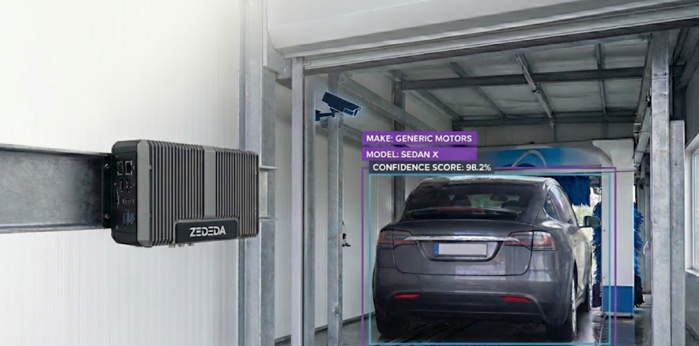
• Object recognition, on the other hand, not only includes detection, but also recognizes object features. For example, what is the make and model of a car? What is its license plate? How large is it?

While object detection is useful for simple tasks, such as opening a gate to a parking lot or garage, it ignores a vast amount of useful information. Imagine if a system could do more than just detect a car; what if it could tell you exactly what kind of car it is?

This is a small shift in perspective, but it unlocks a world of possibilities. When a system can accurately identify a vehicle’s make and model, it transforms from a simple action trigger into an engine for optimization. Think about it:

• Car washes adjust water usage based on vehicle size, reducing water bills and improving profitability.
• Factories perfectly match materials, such as paint, to each model, eliminating waste.
• Toll booths calculate fees based on each vehicle’s emissions and mileage ratings.

These aren’t just minor tweaks; they’re fundamental changes that enhance individual customer experiences and benefit companies and society at large. 

But if fine-grained car recognition is so powerful, why isn’t it everywhere? The truth is, while academic papers showcase high-performing AI models, the real world is far more complex:

1. Feature drift: Deployment environments vary, leading to feature drift in some locations and, in turn, affecting model accuracy there. For example, lighting changes from one car wash location to another, leading to a shift in pixel values. Or even at the same car wash, lighting changes due to the sun being at different angles as the seasons change, and shadows are cast, which can shift pixel values.
2. Device limits: Edge devices have resource constraints around CPU, GPU, and memory. Data scientists not only need to improve the accuracy of AI models, but also achieve it with these constraints, leading them to apply additional techniques on top of these models to make them lighter without losing accuracy.
3. Fleet management: Deploying, managing, monitoring, and updating AI models across a fleet of remote edge devices with limited bandwidth or intermittent network connectivity presents another operational challenge. Sending technicians to manually update each device (truck rolls) is expensive at scale. A machine learning team might be rapidly improving their AI models, but those improved models are useless if they cannot be deployed to remote sites.

Why the Edge? Overcoming the Limits of the Cloud

The “Edge vs. Cloud” debate is extensive, but for powerful AI models, the default assumption is often to run them in the cloud, since the cloud offers essentially infinite scale and processing power. However, for real-time applications in the physical world, constantly streaming video to a distant server creates four major problems that edge computing elegantly solves. They are as follows:

1. Operational Expenses

Cloud computing isn’t free. For vision AI, the highest hidden cost is bandwidth. Continuously uploading high-resolution video from just one camera is like streaming 4K Netflix 24/7. Multiply that by hundreds or thousands of devices, and you can see how these costs will drag down a business’s profitability.

• Cloud Approach: You pay a constant “data tax” for video uploads and cloud GPU processing, leading to unpredictable operational expenses that scale poorly.
• Edge Approach: Data transmission costs are virtually eliminated. Processing occurs on small, power-efficient devices, resulting in a much lower and more predictable Total Cost of Ownership (TCO).

2. Compliance

Continuously sending video feeds of customer cars or public streets to the cloud presents a significant legal liability. This sensitive data needs to be protected, not broadcast. 

• Cloud Approach: Regulated data, such as license plate data and facial scans of car occupants, travels across the public internet, where it is stored on a server, creating multiple points of liability. Collecting this data requires consent in the EU per GDPR and the state of Illinois BIPA. It requires the option for opt-out in California per the CCPA. Capturing video of minors presents compliance risks under GDPR, the UK Children’s Code, and the US COPPA. Navigating this thicket of regulatory requirements means expensive legal bills, friction to the consumer experience, and tricky business logic for software developers to implement.
• Edge Approach: Processing of video happens on an edge device. Raw footage is not transmitted or saved. Only summarized, anonymized results (e.g., “Toyota Camry, Blue, 2024 model year”) leave the device. No complex opt-in or opt-out logic required. You ship faster, your customers have a smoother experience, and you cut out a huge chunk of legal liability.

3. Outages

What happens when a remote site’s internet connection drops or your cloud provider has an outage? If your operation depends on that connection or cloud provider, your business stops. Factories stop running, tolls go uncollected, and so forth.

• Cloud Approach: A car pulls into an automated car wash, but the network is down. The system fails, leading to a stuck customer and lost revenue.
• Edge Approach: The system is self-reliant. The AI model runs locally, identifying the car and starting the correct wash cycle regardless of internet connectivity. For critical infrastructure, “always on” isn’t a feature; it’s a requirement.

4. Latency

You can’t outrun the speed of light. Every time you send data to the cloud, you introduce a delay (latency) for data travel, processing, and response.

• Cloud Approach: A car approaches a smart toll booth. Sending the image to the cloud, processing it, and getting a response takes a few seconds (or sometimes longer), a frustrating pause for the driver.
• Edge Approach: Recognition happens in near real-time, often in milliseconds. The gate opens instantly, providing a seamless user experience. Low latency is essential for safety and efficiency in industrial settings.

By processing AI at the Edge, you build a system that is secure by design, fundamentally more reliable, economically scalable, and instantly responsive. For real-world car recognition, it’s not just the better choice, it’s the only one that truly works. 

As stated above, building an AI application for the edge isn’t just about high accuracy; it’s about achieving it within strict hardware and environmental limits. These constraints often define what’s possible and influence every architectural decision.

At the core, two main factors drive these limitations:

1. Device Capabilities: Edge devices have limited memory, storage, processing speed, and sometimes network bandwidth. The AI model must fit within these constraints without compromising performance.
2. Modularity and Extensibility: The application should be modular, allowing for integration into larger pipelines or extension to related tasks such as license plate recognition, anomaly detection, or traffic analytics.

Since there’s no better way to learn than by doing, let’s embark on an exciting journey: building an image classifier that can tell you the make and model of a car from a single photo. Buckle up as we dive into every step, from the initial spark of an idea to unleashing our creation into the wild. And don’t worry, we promise to keep it fun and straightforward!

In our examples below, we use Intel NUC devices with consumer-grade CPUs (Intel Core Ultra and newer, Intel Core Ultra 5, 7, and 9 families) for this project because they represent hardware that businesses currently deploy, not just developer kits. These devices offer mature software support, readily available AI SDKs, and compatibility with optimization frameworks like OpenVINO, ONNX Runtime, and Nvidia TensorRT. Our development and benchmarking use an ASUS NUC 14 PRO+ with an Intel Core Ultra 7 155H, simulating a realistic mid-to-high-end edge environment for testing optimization strategies in real-world deployment scenarios. Let’s dive in!

 

How to Choose the Right AI Model for the Job

Before diving into specific models, it’s worth reviewing the range of approaches for car make and model recognition at the Edge. Each has its own strengths, weaknesses, and deployment implications.

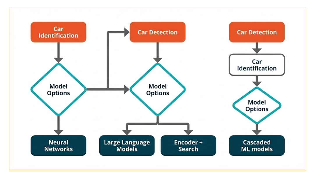
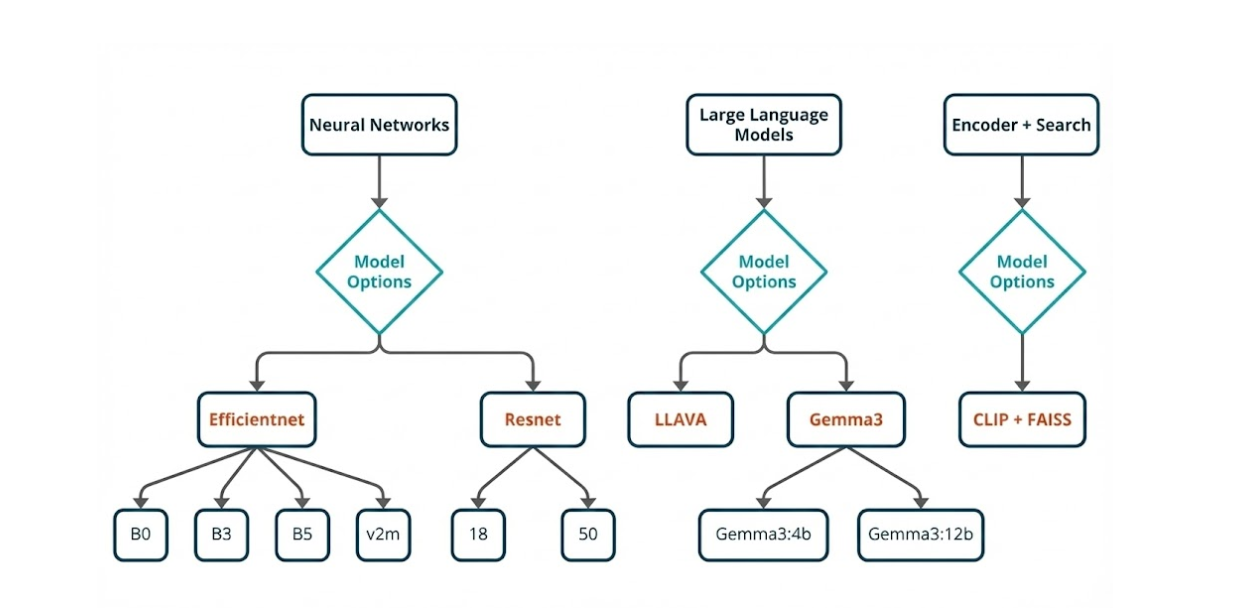
Option 1: Neural Network Classifier

A dedicated image classification neural network (e.g., EfficientNet or ResNet) takes an image of a car and outputs the most likely make and model.

• Strengths: Fast inference when optimized, easy to train, smaller models can run within low-latency constraints, straightforward pipeline.
• Weaknesses: Requires retraining when new makes/models are added. Bear in mind, every year, new car makes and models are introduced.
• Why it’s a strong candidate: Currently, the most accessible approach with abundant tooling, frameworks, pre-trained weights, and well-established edge optimizations.

Option 2: Object Detector + Neural Network Classifier (Cascading)

First, an object detection model localizes the car. Then, the cropped region is fed into a classifier.

• Strengths: Handles images with multiple cars or cluttered backgrounds, improves accuracy in non-ideal camera placements.
• Weaknesses: Two-stage pipeline increases latency, higher resource usage, and difficult to track cascaded errors during deployment.
• When to use: Best suited for environments with numerous objects, and precise localization is crucial.

Option 3: LLM with On-Device Vision Capability

A multimodal large language model (e.g., LLaVA, Gemma with vision) processes images and answers queries about a car.

• Strengths: Highly flexible (descriptions, context), minimal retraining needed (prompt engineering).
• Weaknesses: Large memory and compute footprint, significantly higher latency.
• When to use: For exploratory or multi-purpose assistants, not ideal for high-FPS (frames per second) video streams, or production deployments requiring low latency.

Option 4: Encoder + Search Algorithm

A vision encoder generates image embeddings, which are compared using a vector database and a similarity search engine.

• Strengths: Adding new classes doesn’t require retraining, can handle “one-shot” or “few-shot” learning.
• Weaknesses: Resource-intensive initial vector database creation, requires high-quality embedding space, and can have high inference latency if the database is large.
• When to use: Ideal for large, evolving catalogs where retraining is costly. This fits our car use case, since new makes, models, and color schemes come out yearly.

Choosing the Best Fit for Our Use Case

In terms of adaptability, latency, and deployment simplicity, the neural network classifier (option 1) stands out as the most practical choice for our current scope. Here’s why:

• Retraining Speed: Can quickly go from baseline to production-ready with a single dataset.
• Latency: Can achieve sub-50ms inference on capable edge devices when optimized (such as with FP16 or INT8 quantization).
• Resource Efficiency: Can be packaged into a small container and run with minimal RAM and storage overhead.
• Mature Ecosystem: ONNX Runtime, OpenVINO, and TensorRT all have strong support for convolutional neural network (CNN) classifiers, making deployment smoother.

While encoder + search (option 4) offers long-term scalability without retraining, its higher latency and database management overhead make it less suited for our immediate production goals. LLMs with vision (option 3), while powerful, are currently too resource-intensive for high-speed edge inference. These quotas will vary based on the objective and the environment, so it is important to have fallback solutions for every use case.

Beyond Off-the-Shelf: The Pitfalls of Generic Models

Reusing pre-trained models from public repositories (GitHub, Kaggle, Hugging Face) is attractive, but leaderboard success rarely translates to parking-lot reliability on edge hardware.

Common failure modes and why they matter:

• Class mismatch and regional noise: Public models often cover thousands of vehicle variants, including models never encountered in the target region. Extraneous labels increase confusion and degrade precision for the actual operating catalog.
• Domain shift: Training data rarely match production conditions. Differences in camera optics, mounting height, angle, resolution, weather, motion blur, shadows, and illumination (e.g., infrared at night) can cause significant accuracy drops.
• Granularity gap: Many models stop at coarse categories (“car,” “SUV”). Business logic typically requires fine-grained labels (make → model → year/trim), which generic classifiers do not provide reliably.
• Latency and footprint constraints: Architectures tuned for datacenter GPUs may include operators or tensor shapes that are inefficient on edge runtimes. Without pruning and quantization, inference latency can exceed real-time budgets and memory limits on devices such as Intel Core Ultra NUCs.
• Opaque training provenance: Unknown class balance and curation hide bias. If training skew favors studio imagery, performance on CCTV-style feeds suffers.
• Update friction: Evolving catalogs (new model years, mid-cycle refreshes) demand frequent updates. Generic models lack clean mechanisms for incremental class onboarding and versioned rollouts.
• Pipeline incompatibilities: Differences in preprocessing (resize, color space, normalization) and postprocessing can silently erode accuracy and complicate integration with existing systems.

Implication for Edge deployment

For specifications such as “recognize the most common regional models within a sub-50 ms latency budget on a constrained hardware,” broad, generalist networks are typically over-parameterized, under-optimized, and operationally brittle. Reliable outcomes require a purpose-built model with curated classes, domain-matched data, and edge-first optimizations (INT8/FP16 quantization, supported operators, compact memory footprint). These foundational principles guide our approach to developing robust and efficient recognition systems, as we will explore in the following section on data collection and preparation.

Proposed Solution and System Design

Here’s why we prefer EfficientNet:

• Compound Scaling: EfficientNet scales depth, width, and input resolution jointly, optimizing accuracy for a given compute budget, crucial for fine-grained details within edge latency limits.
• Efficient Building Blocks: mobile inverted bottleneck convolution (MBConv) layers with squeeze-and-excitation offer higher accuracy per parameter, leading to smaller models and lower memory usage at comparable accuracy.
• Edge Performance: EfficientNet variants generally have lower batch-1 latency, a smaller footprint, and stable performance under FP16/INT8 quantization, essential for Intel NUC-class deployments.
• V2 Refinements: EfficientNetV2 improves inference graphs and reduces backend issues in edge runtimes by introducing fused early blocks and training enhancements.

But as good as EfficientNet is, here’s why ResNet remains essential:

• Operational Reliability: Residual blocks use universally optimized operations, such as convolution and ReLU, simplifying export and conversion across ONNX, OpenVINO, and TensorRT.
• Stable Baselines: ResNet-18/34 offer strong latency-accuracy trade-offs for tighter budgets, while ResNet-50 serves as an accuracy benchmark.
• Predictable Quantization: INT8 post-training and quantization-aware training (QAT) are well-understood for ResNet, typically with minimal accuracy impact.

That said, this does not mean other models are not good; they just don’t fit our use case. While other models may offer value, they simply don’t align with our specific needs.

• MobileNet/ShuffleNet: Excellent for ultra-low compute but lacks accuracy for fine-grained distinctions, better suited as early “gates.”
• DenseNet: Competitive accuracy, but higher memory bandwidth and concatenation overhead negatively impact batch-1 latency on edge devices.
• Vision Transformers/ConvNeXt: Strong at scale but demand higher resolution and compute, exhibit more brittle quantization on small devices, and have less predictable latency for real-time applications.

We selected as our primary models EfficientNet B0/B1 (latency-focused), B3/B5 (detail-focused), and EfficientNetV2-M. ResNet-18/34 (latency/memory-focused) and ResNet-50 (accuracy reference) serve as baselines. This choice is based on repeated evaluations on target hardware, prioritizing accuracy within strict latency and memory constraints. EfficientNet is the state-of-the-art for fine-grained vehicle classification at the Edge, complemented by ResNet as a robust and easily deployable baseline. Ultimately, this selection of models forms the foundation for our rigorous testing and deployment strategy, which will be further elaborated upon in the subsequent two sections.

Building Our Foundation: Selecting and Preparing the Data

When you’re building a proof of concept (POC) for an image classification project, the dataset you choose can decide whether your model shines or sinks. And if your goal is to test fine-grained recognition — the kind where details matter — the Stanford Cars dataset is almost tailor-made for the job.

Built for Fine-Grained Challenges

This isn’t just a random assortment of car photos. It’s 16,185 images spanning 196 different classes, each tagged by make, model, and year. That means your model isn’t just learning “this is a car” — it’s learning to tell a 2012 BMW M3 Coupe from its 2013 sibling, a subtlety that forces your network to pick up on real, often tiny visual cues.

For a POC, this kind of detail is gold. It tells you quickly whether your architecture can actually capture nuance — a skill that separates toy demos from real-world solutions.

Dataset Selection and Preparation

The Stanford Cars dataset hits the sweet spot for prototyping: large enough for meaningful results, yet small enough for rapid iteration on a single GPU or CPU on an edge device. It has just the right complexity:

• Intra-class similarity: Challenges the model to spot tiny differences between models and trim levels.
• Inter-class variation: Ensures it learns broader, distinctive features that cut across manufacturers and models.Instant Benchmarks & Plug-and-Play: With existing baseline results from ResNet, EfficientNet, and Vision Transformers, you can immediately compare the results with your reference model. Plus, the clean, ready-to-use format (JPEG images, labels) makes integration with modern architectures frictionless.

• Edge-Ready & Real-World Relevant: Perfect for testing quantization and compression techniques without sacrificing result meaning. If your project touches anything automotive, this dataset mirrors your target environment, ensuring your pipeline will generalize beyond the lab.

Conquering Real-World Variability: How We Augment Data for Robust Models

In the unpredictable real world, data is rarely pristine and uniform. To train AI models that can handle this messy reality, we employ a powerful technique: on-the-fly data augmentation. Before our images even hit the network, we transform them, achieving two critical goals: standardizing inputs for consistent feature extraction and introducing realistic variations to handle diverse cameras, angles, and lighting conditions.

Here’s a peek into our augmentation pipeline, designed to make our models truly robust:

Standardization & Input Shape: Getting Consistent

First, we bring all images to a consistent size. We resize them to 256×256 pixels, then apply a random crop of 224×224. This step not only ensures a uniform input size for our network but also introduces minor framing shifts, encouraging the model to learn features that aren’t tied to precise object placement.

Geometric Variability: Simulating Different Views

To mimic the diverse perspectives a model might encounter, we introduce geometric variations:

• Random Horizontal Flip (p=0.5): Imagine a car driving from left to right, then right to left. This simple flip accounts for different driving directions.
• Random Rotation (±15°): For slight tilts or camera angles, we randomly rotate images up to 15 degrees in either direction.
• Random Affine (translate 10%, scale 0.9–1.1): This allows for slight zooms in and out, and minor framing adjustments, reflecting variations in camera distance.
• Random Perspective (p=0.3): To simulate angled views, we randomly apply perspective transformations, making the model robust to objects seen from various corners.

Photometric Variability: Adapting to Light and Sensor Differences

Real-world lighting is never constant, and different cameras have different sensor characteristics. Our ColorJitter operation tackles this by adjusting brightness, contrast, saturation, and hue. The magic here is that it simulates sensor and lighting differences without losing the crucial, class-defining colors.

Tensor Conversion & Normalization: Setting Up for Success

Before feeding the data to our neural network, we convert the images to tensors and apply ImageNet mean and standard deviation normalization. This crucial step ensures faster, more stable convergence during training.

Validation Pipeline: Honest Assessment

While augmentation is vital for training, we need an unbiased way to assess our model’s true learning. For validation, we use a deterministic pipeline: simple resizing followed by normalization, with no augmentation. This provides a clean and accurate measure of model performance.

Why This Recipe Works

It’s a balanced cocktail of geometry and color tweaks — enough to mimic real-world noise without breaking semantic meaning. Multiple mild transformations stack to create diversity safely, and deterministic validation means your metrics are trustworthy.

Baseline Model Training and Evaluation

Car make and model identification is a fine-grained image classification problem. Unlike general object recognition (e.g., “car vs. bus”), it requires distinguishing between highly similar vehicle types (e.g., a 2018 Toyota Corolla vs. a 2020 Toyota Corolla).

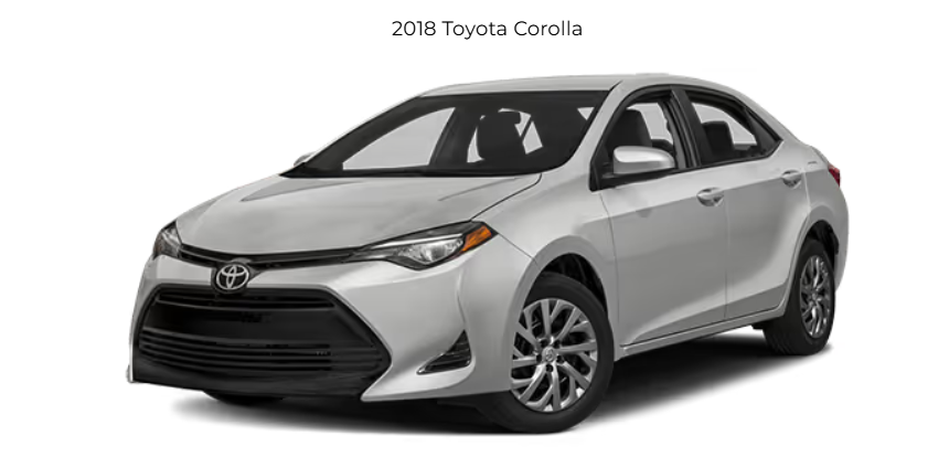
The challenge lies in handling subtle visual cues such as grille shape, headlight design, and body curvature while remaining able to accommodate variances in lighting, angles, and occlusion.

To tackle this, the choice of backbone model is critical. Below, we compare EfficientNet (B3, B5, V2-M), ConvNeXt, and ResNet-50 — five popular CNN architectures — in terms of architecture design, efficiency, and suitability for fine-grained classification tasks like car recognition.

 

Model	Number of parameters	Architectural Deep Dive	Why It Shines for Car Recognition	The Catch (Trade-off)
EfficientNet B3	12 million	A nimble, speed-optimized design with solid accuracy.	Excellent at grasping both broad strokes and minute details, making it a star for real-time edge inference.	Scaling up to higher versions demands significantly more memory and computational muscle, posing limitations for embedded systems.
EfficientNet B5	30 million	A deeper, wider architecture built for performance.	Delivers impressive results on GPUs, ideal for large-scale, cloud-based recognition tasks.	Like its B3 sibling, higher versions are memory and compute-hungry, challenging for constrained embedded environments.
EfficientNetV2-M	54 million	The second iteration of EfficientNet features innovative Fused-MBConv layers (early layers are convolution-heavy, later layers utilize lightweight inverted residual blocks). This design boosts training speed and efficiency.	Boasts faster training times, handles high-resolution images with ease, and is more resilient to real-world visual distortions.	Heavier than EfficientNet B3 and not quite as efficient as ConvNeXt for devices with severe constraints.
ConvNeXt Base	89 million	A modern CNN that draws inspiration from Vision Transformers (ViTs). It maintains a CNN backbone but integrates transformer-like elements such as large kernel sizes, layer normalization, and simplified residual blocks.	Superb at understanding long-range dependencies, competing head-to-head with transformer-based models. Delivers strong performance on high-resolution datasets and is simpler to train and fine-tune than ViTs.	Generally heavier than EfficientNet B3 and ResNet-50, potentially making it less ideal for direct edge deployment without optimization techniques like quantization or pruning.
ResNet-50	26 million	A foundational CNN known for its residual connections (skip connections that combat vanishing gradients during training).	Comparatively lightweight next to ConvNeXt or EfficientNet-B5; a proven and dependable choice for feature extraction; a vast library of pretrained weights and variations is readily available.	Struggles to distinguish fine-grained differences when pitted against newer architectures; its smaller receptive field, compared to ConvNeXt or EfficientNetV2, can lead to reduced accuracy on subtle distinctions like the shape of taillights.

 

From Model to Milliseconds: Optimizing Inference on Edge Hardware

A trained model is only a starting point. To be useful in a production environment, it must perform inference within strict time budgets. On resource-rich cloud servers, low-level optimization can sometimes be overlooked; at the Edge, it is non-negotiable.

Our target application involves processing live video feeds. Doing so sets a clear baseline for performance: to avoid stuttering or missed frames, we must achieve a throughput of at least 24 frames per second (FPS). For more demanding scenarios, such as high-speed monitoring or enhanced user experiences, the target can climb to 30 or even 60 FPS.

Achieving this leap in performance isn’t about brute force. It’s about intelligent workload distribution. In this case, it requires a two-pronged approach:

Model-Level Optimization: Making the neural network itself smaller, faster, and more computationally efficient.

Deployment-Level Optimization: Intelligently dispatching the optimized model to the specialized hardware accelerators available on the device.

Model-Level Optimization Techniques

Before the model ever touches the hardware, we can dramatically reduce its size and complexity with several techniques.

Model Quantization: This process reduces the numerical precision of the model’s parameters (weights and activations). Most models are trained using 32-bit floating-point numbers (FP32). Quantization converts these to a lower precision, such as 16-bit floating-point (FP16) or, more commonly, 8-bit integers (INT8).

Impact: INT8 quantization can reduce model size by up to four times and significantly accelerate inference speed, as integer arithmetic is much faster than floating-point math on many modern CPUs and is the native format for NPUs. This comes at the cost of a minor, often negligible, drop in accuracy.

Other methods that are effective that we won’t be covering in this blog include:

Model Pruning: This technique involves identifying and systematically removing redundant or unimportant parameters (individual weights or entire neurons) from the network. Many large neural networks are heavily over-parameterized, and pruning can reduce their size and the number of calculations required for a forward pass.

Impact: Pruning creates a smaller, “sparser” model that is faster and more memory-efficient. This process typically requires a fine-tuning step after pruning to restore any accuracy lost by removing the parameters.

Knowledge Distillation: An advanced technique where a large, highly accurate “teacher” model is used to train a much smaller, faster “student” model. The student learns to mimic the teacher’s outputs, effectively compressing the learned knowledge into a more efficient architecture.

By applying these techniques, we transform a large, cumbersome model into a lean, efficient asset ready for the edge.

Deployment-Level Optimization via Hardware Acceleration

Once the model is lean, the next step is to execute it on the most suitable hardware component. Modern edge devices like our Intel NUC are Systems-on-a-Chip (SoCs) with multiple specialized compute units.

On our ASUS NUC 14 PRO+ with its Intel Core Ultra processor, we have three primary targets for inference:

CPU (Central Processing Unit): Serves as our performance baseline and is excellent for complex models with operations not supported by other accelerators.

iGPU (Integrated Graphics Processing Unit): A parallel processor ideal for floating point matrix multiplication and convolution operations common in neural networks.

NPU (Neural Processing Unit): A dedicated, low-power AI accelerator. First introduced in Intel’s Core Ultra processors (code-named “Meteor Lake”), the NPU is purpose-built for sustained, energy-efficient AI inference. Its architecture is optimized for integer matrix multiplication, and thus quantized (INT8) models, making it a good match for our model-level optimizations.

Post-Optimization Results and Trade-Offs

With our candidate models selected and trained, let’s go to the first phase of optimization: post-training quantization (PTQ). The goal is to convert the models from their 32-bit floating-point (FP32) precision to 8-bit integers (INT8) and measure the impact on three key metrics:

1. Accuracy (%): How much did performance drop after quantization?
2. Latency (ms): How much faster is the model? (Lower is better).
3. Model Size (MB): How much smaller is the model on disk?

The following benchmarks were run using the ONNX Runtime on our testbench’s CPU (Intel Core Ultra 7 155H) to establish a consistent baseline before moving to other hardware accelerators.

Model Family	Precision	Accuracy	⏱️ Avg. Latency (ms)	💾 Size (MB)
ResNet50	FP32 (Baseline)	89.39%	398.45 ms	94.0 MB
	INT8 Dynamic	88.53%	698.59 ms	23.7 MB
	INT8 Static	89.14%	121.66 ms	23.7 MB
EfficientNetB3	FP32 (Baseline)	89.42%	348.09 ms	44.1 MB
	INT8 Dynamic	0.27%	2262.28 ms	11.6 MB
	INT8 Static	0.40%	248.79 ms	11.8 MB
EfficientNetB5	FP32 (Baseline)	89.62%	600.66 ms	112.4 MB
	INT8 Dynamic	0.62%	4410.32 ms	29.1 MB
	INT8 Static	35.38%	390.38 ms	29.4 MB
EfficientNetV2-M	FP32 (Baseline)	89.18%	766.45 ms	204.2 MB
	INT8 Dynamic	70.84%	3362.63 ms	52.4 MB
	INT8 Static	61.76%	351.90 ms	52.8 MB
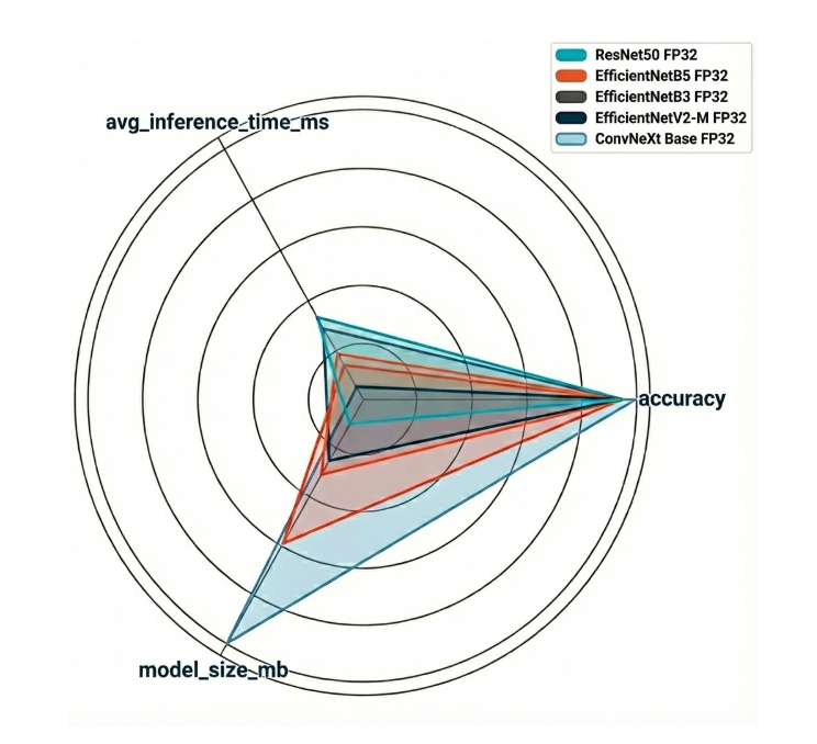
ConvNeXt Base	FP32 (Baseline)	93.78%	1706.25 ms	336.6 MB
	INT8 Dynamic	93.73%	6294.02 ms	85.0 MB
	INT8 Static	93.07%	2090.16 ms	85.0 MB

Key Analysis and Observations

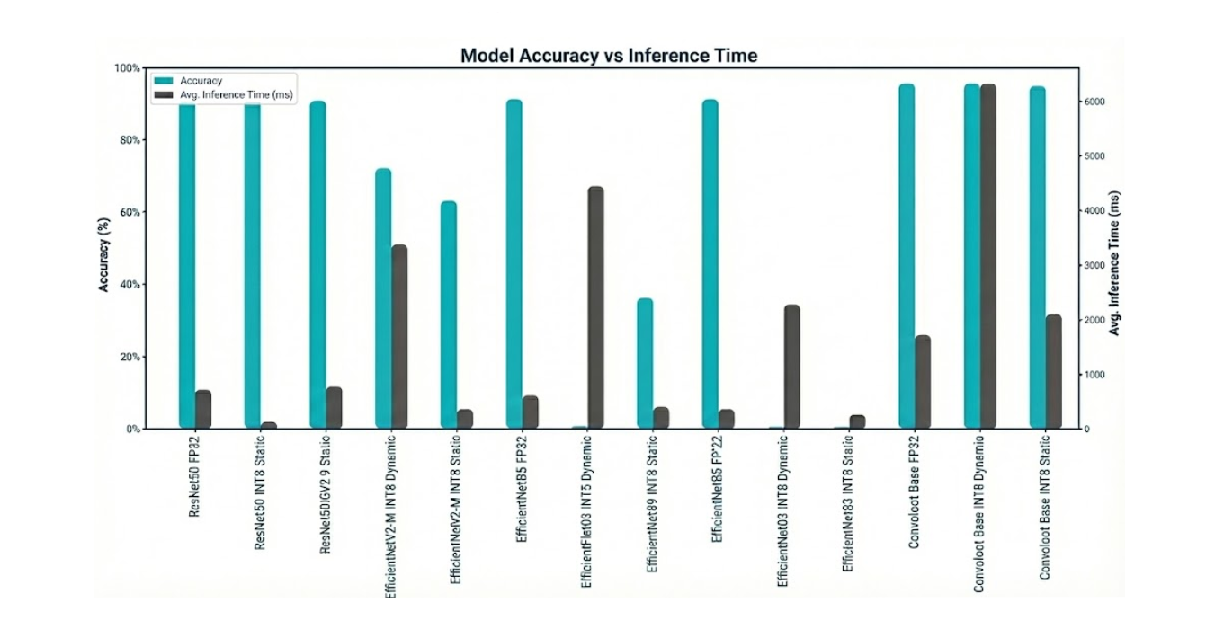
1. The Power of Static Quantization (When it Works): The ResNet50 model is a textbook example of successful quantization. With static INT8 quantization, we achieved a 3.3x speedup (398ms → 121ms) and a 4x reduction in model size, all while losing a negligible 0.25% of accuracy. This is the ideal outcome for edge optimization.
2. The Peril of Dynamic Quantization: Across all models, INT8 Dynamic quantization proved to be a performance trap. Because it calculates quantization ranges on-the-fly for each activation during quantization, the lack of calibration and stateful training made it significantly slower than the FP32 baseline in every case. This technique is not suitable for low-latency inference.
3. Not All Architectures Quantize Equally: The EfficientNet family of models demonstrates a critical risk of Post-Training Quantization. The B3 and B5 variants experienced a catastrophic drop in accuracy, rendering them completely unusable after conversion to INT8. This highlights that certain architectures are more sensitive to reduced precision, and that validation after every optimization step is non-negotiable.
4. The Accuracy vs. Latency Trade-Off: The ConvNeXt Base model delivered the highest accuracy of all candidates at 93.78%. However, its FP32 latency of over 1.7 seconds (roughly 0.6 FPS) makes it entirely unsuitable for our real-time requirements. Even after quantization, it remained over 2 seconds. This is a classic engineering trade-off: the most accurate model is not always the best model for the job.

Model Comparison & Final Recommendation

Based on the benchmark results, we can immediately eliminate several candidates:

• The entire EfficientNet family (B3, B5, V2-M). Their inability to withstand post-training quantization without a severe loss of accuracy makes them too brittle for this production pipeline.
• ConvNeXt Base. Despite its superior accuracy, its latency is an order of magnitude too high for any real-time application.

This leaves us with a clear winner that excels across all three of our key criteria for an edge deployment.

Our Final Recommendation: the ResNet50-INT8-Static model with INT8 Static Quantization is the standout choice for our on-device vehicle recognition system.

Here’s why it’s the best fit:

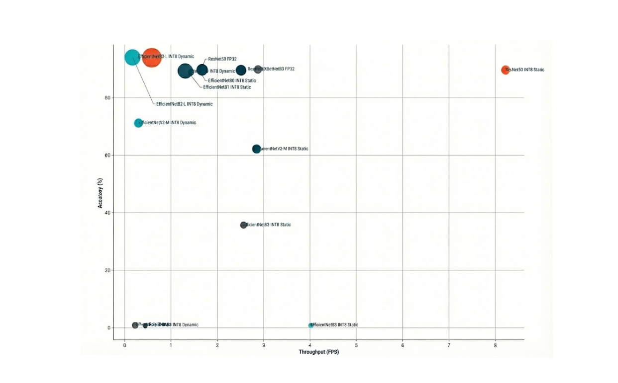
• Balanced Performance: Its CPU baseline latency of 122 ms (~8 FPS) is the fastest starting point among all tested models. While this doesn’t yet meet our 24 FPS target, it provides the best foundation for further acceleration on the iGPU and NPU.
• High Accuracy & Robustness: With 89% accuracy, it delivers reliable, trustworthy results. Crucially, it demonstrated robustness by maintaining this accuracy throughout the quantization process.
• Excellent Efficiency: At just 24 MB of disk space, the model has a tiny footprint, making it easy to deploy, update, and manage on resource-constrained devices. It consumes minimal RAM and storage, leaving resources available for other applications running at the Edge node.

In conclusion, the ResNet50 architecture, when optimized with static INT8 quantization, provides the ideal blend of speed, accuracy, and efficiency. The next and final step is to take this optimized model and offload its execution to the iGPU and NPU to smash our 24 FPS performance target.

 

 

 

Accuracy versus Throughput (bubble size = model size)

Normalized Model Comparison Heatmap

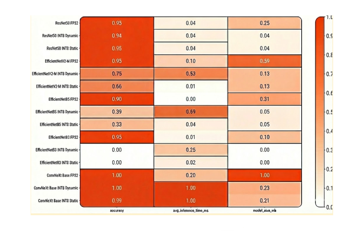
Packaging for Production: Containerization and Helm Charts

Containerizing the Application for Deployment

Now lets transform our trained model into a reliable system that can run on edge devices with minimal manual intervention.

Goals:

• Small and Secure Docker Images: To ensure fast startup times and reduce the attack surface for increased security.
• Kubernetes Helm Chart: For repeatable, parameterized, and easily upgradable deployments of models and code.
• Automatic Model Updates: To allow new model versions to be deployed without rebuilding the entire image. Remember, new car models are continually coming onto the market and need to be recognized by our system.

The Three-Container Architecture

The system is divided into three containers, each with a distinct responsibility:

• Inference Server: Runs the model in production. This setup utilizes OpenVINO Model Server (OVMS), which supports both gRPC (port 9000) and REST (port 8000) for predictions.
• Model-Sync Sidecar: Periodically checks an object storage service (e.g., MinIO or Amazon S3) for new model files. Upon discovery, it downloads the file into a shared folder and triggers the server to reload.
• Client / Business Logic: A small tool useful for testing and demonstrating the system during development, but should be disabled in production. In a production environment, this component will house the customer’s business logic, including scripts and methods that can be requested from the server.

Best Practices for Production

• Small Base Images: Lightweight Docker images like Python:slim are used to keep things efficient.
• Non-Root Execution: All containers run as non-root users to enhance security.
• Locked-Down Package Versions: Build processes ensure specific package versions are used for consistent, predictable execution.
• Extra Metadata: Images include additional metadata such as:
  • Build timestamp
  • Git commit SHA
  • Model version number

Health Checks and Configuration

• Liveness Probes: Verify if the server process is still running.
• Readiness Probes: Confirm if the model is loaded and prepared for predictions.
• Configuration Management: Configuration files are stored in Kubernetes ConfigMaps, while credentials are kept in Kubernetes Secrets, ensuring they are not embedded within the container image.

Filesystem and Model Lifecycle

• Shared Volume: A Kubernetes PersistentVolumeClaim (PVC) is mounted at /models and shared between the server and sidecar.
• Structured Directory Tree: When the sidecar downloads a model, it places it in a structured directory: /models/<model_name>/<version>/
• Hot Reloading: The inference server monitors this folder and hot-reloads the model when changes are detected. Hot reloading means that only the model is reloaded into memory, and nothing else.

Performance and Networking

• Resource Limits: Prevent one service from consuming excessive resources and impacting others.
• Model Optimization: Models are optimized to INT8 to reduce startup time and memory usage.
• Networking: Networking is internal by default (ClusterIP) but can be exposed externally if required.

Observability

• Structured Logs: All logs are formatted in JSON for easier parsing.
• Metrics Endpoint: A /metrics endpoint is exposed for monitoring tools like Prometheus.
• Reload Information: The system logs important information, including model version and checksum, upon every reload.

 

How to Manage the Fleet at the Edge

Here’s our rationale behind our Helm chart design. At their core, Helm charts embody a modular, production-first design philosophy. It is not just a packaging of Kubernetes manifests. It involves:

1. Separation of Concerns

Our Helm chart deliberately splits the system into distinct roles:

• Inference Server (OpenVINO Model Server) – The heart of the system, exposing gRPC and REST endpoints for predictions.
• Model-Sync Sidecar – A lightweight companion that continuously checks object storage (e.g., AWS S3, MinIO) for updated models and hot-reloads them without downtime.
• Client Deployment – An optional component for testing or demo purposes. In production, this can be swapped with customer-specific business logic.

This separation ensures that the inference pipeline is not monolithic but composable, making it easy to maintain and upgrade parts independently.

2. Automation as a First-Class Citizen

One standout idea is automatic model lifecycle management. Instead of baking models into container images, our chart externalizes them. The sidecar container automates fetching, syncing, and refreshing models, enabling teams to deploy new versions rapidly without redeploying the entire infrastructure.

This philosophy aligns with modern MLOps practices: decoupling code from model artifacts so teams can iterate faster.

3. Security and Minimalism

The chart enforces Kubernetes best practices:

• Uses non-root containers and fine-grained serviceAccount definitions.
• Keeps Docker images minimal (we recommend distroless images, specifically ubi-minimal).
• Encourages locked package versions and traceability through labels (git SHA, model version, build timestamp).

These choices reduce the attack surface and make the system easier to audit.

4. Scalability and Observability

The inclusion of Horizontal Pod Autoscaling (HPA) and configurable resource limits reflects the philosophy that inference workloads must adapt to varying traffic. The design anticipates spikes in requests and ensures performance without manual intervention.

We’ve built in health probes and ingress configurations, making our system production-ready from day one.

5. Flexibility via Values

Through values.yaml files and environment-specific variants (values-dev.yaml, values-prod.yaml), we’ve designed our Helm chart to be portable across deployment scenarios. The same Helm chart can target, a developer’s laptop running minikube, a  staging environment on Kubernetes, or a production cluster orchestrating workloads at the edge or in the cloud.

 

This reflects the idea of “build once, run anywhere” for ML inference. Once the containers and Helm charts are ready, ZEDEDA handles orchestration and rollout to edge devices.

1. Pre-Deployment Checklist:

• Images are pushed to a container registry.
• Secrets are created for object storage and TLS certificates.
• PVCs are sized correctly for model storage.
• Node labels match the target hardware (e.g., Intel NUC).

2. Testing Before Deployment

In your terminal, render the Helm chart with your site-specific configuration:

 

3. Run it in a local cluster (k3s, kind, or minikube) to check:

• Pods are in the Ready state.
• Models load correctly.
• Health checks pass.
• A test prediction works.

4. Packaging the Helm Chart

Lint, package, and version it in your terminal:

5. Keep a CHANGELOG to track:

• Image tags
• Model versions
• Schema or label changes

6. Rolling Out in ZEDEDA

• • Upload or reference the Helm package in ZEDEDA Kubernetes Marketplace.
  • Create the application definition and provide site-specific settings.
  • Target your edge devices and define placement policies.

  Deploy and wait for the system to report Ready.
  

7. Post-Deployment Verification

• Send a test request to confirm predictions work.
• Check metrics and logs to confirm the model version is correct.
• For updates, either:
  • Push a new model to storage (sidecar will sync it), or
  • Update the image tag in the chart.

8. Ongoing Operations

• Model updates: Push to storage → Sidecar downloads → OpenVINO model reloads → Smoke test.
• Rollbacks: Point back to an older model version or chart values.
• Monitoring: Watch for changes in latency, memory, or accuracy — use a canary rollout for safety.

This workflow ensures that your AI models can run reliably at the edge with minimal downtime, secure credential handling, automatic updates, and centralized fleet management through ZEDEDA. Once in place, it’s a predictable, repeatable process for deploying, monitoring, and upgrading models without interrupting service.

How to Deploy AI Apps and Models with ZEDEDA

With our application packaged as a containerized, Helm-defined workload, the ZEDEDA platform takes over to handle the unique complexities of edge orchestration. ZEDEDA is the control plane that bridges our application to the distributed fleet of physical edge devices. To do this, we use ZEDEDA Edge Kubernetes App Flows, documented here, to deploy our applications and models to our edge devices.

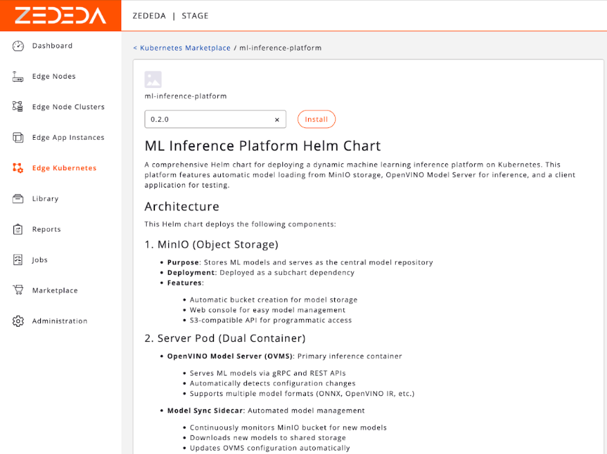
First, we upload our container images and Helm chart to ZEDEDA’s cloud-based controller. Then we define a “Project” and specify which device group (e.g., “all-california-stores,” “factory-floor-line-1”) should run this application. Once we’ve uploaded it, we should see it in our ZEDEDA Kubernetes Marketplace; the screenshot below shows one such chart called ml-inference-platform.

 

If we double-click on that Helm chart, we’ll see its readme.md, explaining its contents so your other teammates know more about it and how to use it.

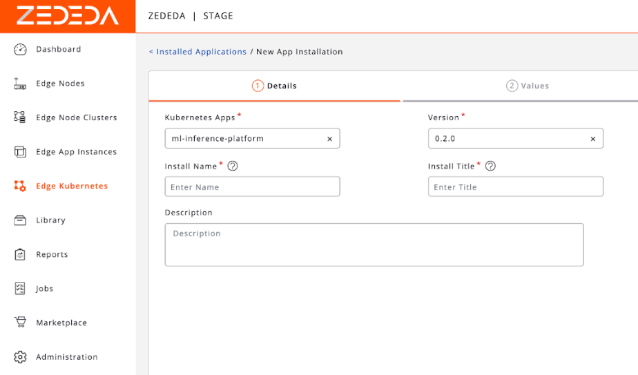
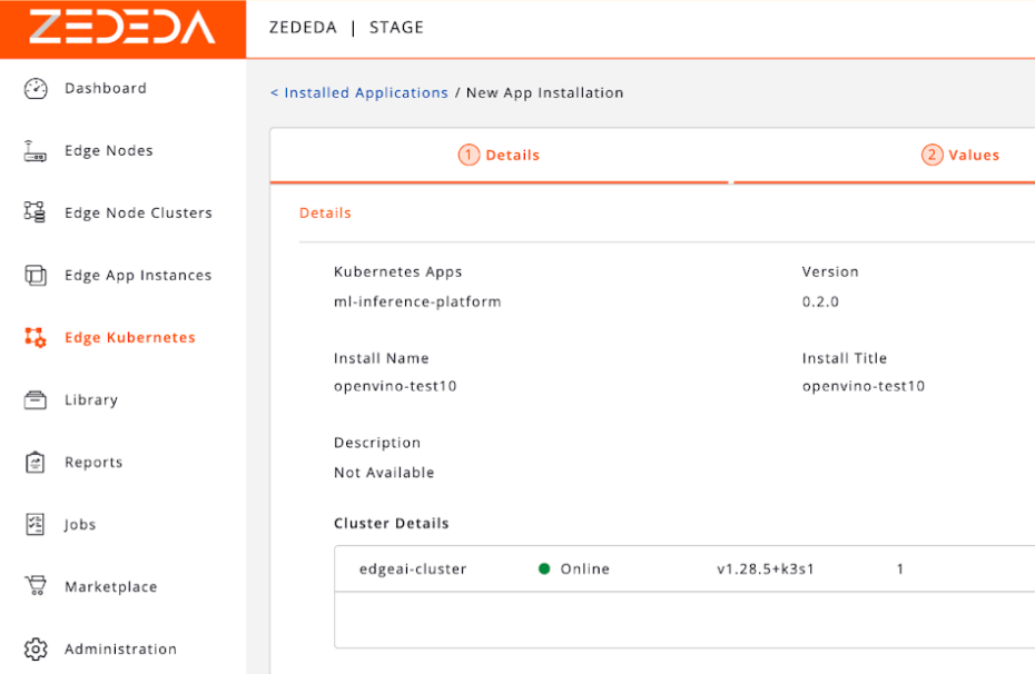
We can specify metadata about the application, such as its version, install name and title, and description.

 

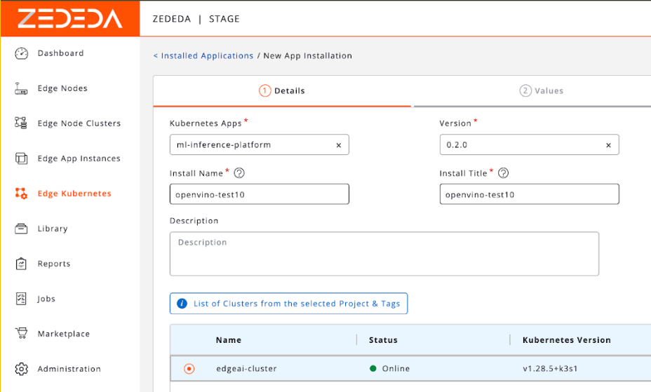
We can then specify which clusters we want to install this app into. For example, this could be clusters of edge devices at retail stores, or remote oil well sites.

 

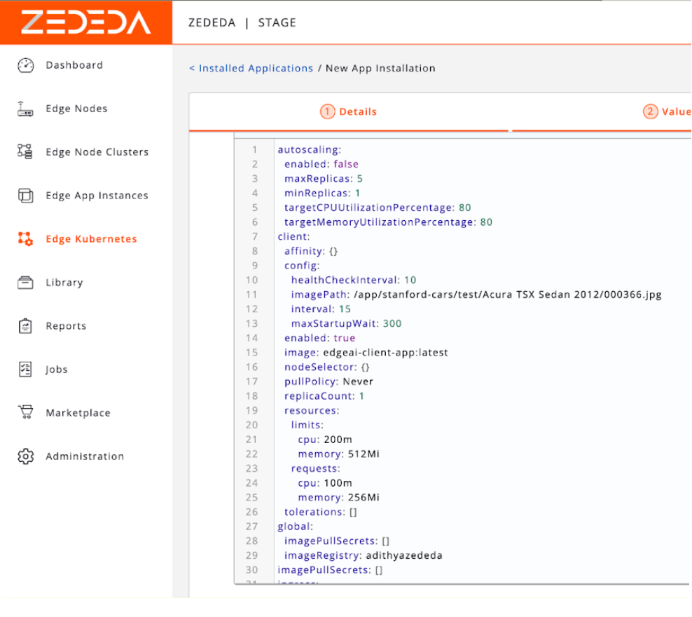
After we click on our cluster, we can change its configuration options and edit its YAML.

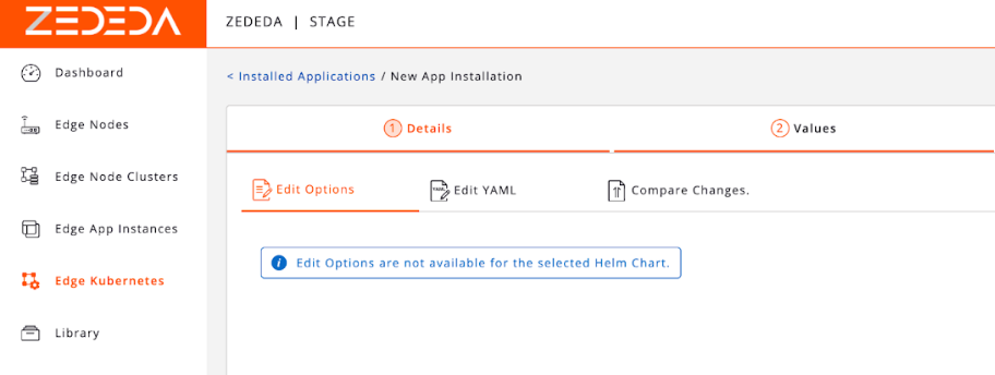
We have a built-in YAML editor, giving you fine-grained configuration control.

 

Once the configuration has been finalized, you can install the application into ZEDEDA Cloud.

 

 

Once the application is installed into ZEDEDA Cloud and scheduled for deployment, ZEDEDA then automatically handles the entire rollout of your app and model to edge devices:

• Secure Provisioning: The ZEDEDA agent on each edge node securely connects to the central controller.
• Container Deployment: It pulls the specified container images and Helm configuration.
• Application Orchestration: It starts the application services as defined in the chart, ensuring all containers are running and healthy.

Key Orchestration Features

This is where the power of a true edge orchestration platform becomes clear.

• Zero-Touch Model Updates: To update our vehicle recognition model, we simply upload the new example-model.onnx file to our S3 bucket. The model-sync sidecar on every single device in the fleet sees the new version, downloads it, and hot-reloads the inference server. The update is deployed globally in minutes, with zero manual intervention and zero downtime.
• Atomic Application Upgrades: To update the core application itself (e.g., moving to a new version of the OpenVINO Model Server), we upload a new version of the Helm chart to ZEDEDA. The platform then orchestrates a rolling update across the entire fleet, ensuring the application is upgraded safely and consistently everywhere.

Monitoring, Logging, and Alerting

ZEDEDA provides a single pane of glass for the health of the entire fleet. We can monitor resource consumption (CPU, memory, storage) for every device and application from its central cloud controller. Logs from all containers are streamed back to ZEDEDA Cloud, allowing us to debug issues on a device thousands of miles away as if it were sitting on our desk.

This centralized control transforms the operational challenge of managing a distributed network of AI-powered devices from an impossible task into a routine, automated process. It allows us to focus on improving our AI while ignoring backend orchestration.

 

Conclusion and What’s Next: The Future is on the Edge

The journey from a simple idea—identifying a car’s make and model—to a robust, scalable edge AI solution is a testament to the power of a holistic engineering approach. We’ve demonstrated that success in the real world isn’t just about leaderboard-topping model accuracy. It requires a deliberate, multi-stage process:

• Strategic Selection: Choosing an architecture like ResNet50 that balances high performance with proven robustness.
• Rigorous Optimization: Applying techniques like INT8 static quantization to create a model that is lean, fast, and efficient.
• Hardware-Aware Deployment: Leveraging specialized silicon like Intel’s iGPU and NPU through toolkits like OpenVINO to meet demanding real-time performance targets.
• Cloud-Native Orchestration: Packaging the entire system with Helm and managing the fleet with a platform like ZEDEDA to achieve true operational scale.

Our final solution—a quantized ResNet50 model, served by the OpenVINO Model Server and deployed via a modular Helm chart—is more than just a proof of concept. It is a production-ready blueprint for delivering high-performance computer vision at the edge, capable of deployment and management across a global fleet of devices, with security, reliability, and automation at its core. 

Future Enhancements

While our current solution is powerful, this is just the beginning. The modular architecture allows for continuous improvement and expansion. Here are the next steps on our roadmap:

1. Unlocking the NPU: Our next performance deep-dive will be to benchmark this workload specifically on the Intel Core Ultra’s Neural Processing Unit (NPU). The goal is to quantify the performance-per-watt advantage of this dedicated AI accelerator, which is critical for power-constrained or thermally sensitive deployments.
2. Advanced Optimization with Quantization-Aware Training (QAT): For models that show accuracy degradation with Post-Training Quantization (such as the EfficientNet family), QAT is the next logical step. By introducing the simulation of quantization effects during the training process itself, QAT can often produce an INT8 model with virtually no accuracy loss, potentially making these highly efficient architectures viable for production.
3. Data Feedback Loop: Using ZEDEDA, we can configure the system to capture low-confidence predictions from edge devices and securely upload those images to a central data store. This “hard-case mining” will provide an invaluable, ever-growing dataset for retraining and refining our model, ensuring it adapts and improves over time.

The future of AI is at the edge, and by combining intelligent model optimization with powerful orchestration, we can turn cutting-edge research into tangible, operational value.

Next steps

If you want to build Edge AI object recognition, whether for cars or other types of objects, ZEDEDA can help. We deliver a complete, on-device solution that transforms this powerful recognition capability from a research concept into a scalable, operational reality. Our mission is to move these promising AI capabilities out of the cloud and put them to work in the physical world. We’ve built a real-time, on-device AI solution, managed at scale by our edge orchestration platform, making fine-grained vehicle recognition practical, profitable, and ready for production. Get in touch at https://zededa.com/contact-us/. 

 

FAQ

Frequently Asked Questions: AI for Vehicle Recognition at the Edge

1. What is the business value of identifying a car’s make and model instead of just detecting its presence?

Moving beyond simple presence detection to fine-grained classification unlocks significant business value. For example, a system that can identify a vehicle’s make and model can enable:

• Car washes adjust water usage and materials based on the vehicle’s size and model, reducing waste.
• Painting facilities to perfectly match materials to specific models.
• Smart toll booths to calculate fees based on factors like a vehicle’s emissions profile. This transforms a simple trigger into an engine for optimization, enhancing customer experiences and operational efficiency.

 

2. Why should I run my AI model on an “edge” device instead of in the cloud?

While the cloud offers immense processing power, running real-time AI for physical-world applications on the edge solves four critical problems:

• Lower Costs (TCO): Edge computing virtually eliminates the high, ongoing bandwidth costs of streaming high-resolution video to the cloud. Processing on small, power-efficient devices leads to a more predictable and lower Total Cost of Ownership (TCO).
• Low Latency: Processing occurs in milliseconds on the local device, providing an instant response. This is essential for safety, efficiency, and a seamless user experience, such as a toll gate opening immediately for a car.
• Reliable Operations: The system can function without a constant internet connection. This ensures reliability for critical operations, preventing downtime if the network fails.
• Privacy & Security: Processing happens locally on the device, so sensitive video footage is not continuously sent over the internet. Only encrypted results (e.g., “Toyota Camry, Blue”) leave the device, minimizing data vulnerability and compliance overhead.

 

3. Can’t I just use a powerful, pre-trained model from a public repository like Hugging Face?

Using off-the-shelf, generalist models for specific edge deployments is often unreliable. These models typically fail in production for several reasons:

• Domain Shift: They are trained on data that doesn’t match real-world production conditions, like different camera angles, lighting, weather, or motion blur.
• Class Mismatch: They often include thousands of vehicle variants not found in your target region, which can confuse the model and reduce precision.
• Performance Constraints: Architectures designed for powerful datacenter GPUs are often too slow and memory-intensive for resource-constrained edge hardware like an Intel NUC.
• Lack of Granularity: Many generic models only identify coarse categories like “car” or “SUV,” not the fine-grained make and model needed for business logic. For a reliable edge application, a purpose-built model with curated data and edge-first optimizations is required.

 

4. What kind of AI model architecture is best for this task?

For real-time vehicle recognition at the edge, a Neural Network Classifier (like ResNet or EfficientNet) is the most practical choice. While other approaches exist, this one offers the best balance of:

• Low Latency: When optimized, these models can achieve sub-50ms inference times on capable edge devices.
• Resource Efficiency: They can be packaged into small containers with minimal RAM and storage overhead.
• Mature Ecosystem: There is strong tooling support from frameworks like OpenVINO, ONNX Runtime, and TensorRT, which simplifies optimization and deployment. Architectures like Vision Transformers (ViTs) and ConvNeXt, while powerful, often demand more compute resources and can have less predictable latency on small devices.

5. How do you make a large AI model small and fast enough to run on an edge device?

Making a model “edge-ready” requires a two-pronged optimization strategy:

1. Model-Level Optimization: This involves making the model itself more efficient. The key technique is Model Quantization, which converts the model’s parameters from 32-bit floating-point numbers (FP32) to more efficient 8-bit integers (INT8). This can reduce model size by up to 4x and significantly speed up inference, especially on hardware with dedicated AI accelerators (NPUs).
2. Deployment-Level Optimization: This involves using the specialized hardware on the edge device. Modern Systems-on-a-Chip (SoCs) include a CPU, an Integrated GPU (iGPU), and a Neural Processing Unit (NPU), each optimized for different tasks. By using frameworks like OpenVINO, the optimized model can be run on the most suitable accelerator to achieve performance targets like 24+ frames per second (FPS).

 

6. I’ve optimized my model. How do I deploy and manage it across hundreds or thousands of devices?

Managing a fleet of edge devices requires a cloud-native orchestration platform like ZEDEDA. The workflow involves:

• Containerization: The application is packaged into containers, often with a Helm chart for repeatable and configurable deployments. The architecture might include separate containers for the inference server, a “model-sync sidecar,” and business logic.
• Centralized Deployment: Container images and Helm charts are uploaded to the ZEDEDA controller. From there, you can define which device groups should run the application and roll it out automatically.
• Zero-Touch Updates: Model updates are automated. You simply upload a new model file to a cloud storage bucket (like S3), and the sidecar on each device automatically downloads it and hot-reloads the server with zero downtime. Application upgrades are handled similarly by uploading a new Helm chart.
• Monitoring and Logging: The platform provides a “single pane of glass” to monitor the health and resource consumption of every device and stream logs back to a central location for debugging.