A technical deep-dive into the ZEDEDA Camera Monitoring Agent for PCB Quality Inspection at the Edge using NVIDIA Jetson Thor
Summary
Modern electronics manufacturing demands sub-millimeter defect detection at production line throughput, yet the AI models that power such systems are notoriously brittle in the face of environmental drift, board variant changes, and evolving defect taxonomies. The conventional response of retraining the model is expensive, slow, and operationally disruptive. This paper presents an alternative: an agentic vision system that separates the perception layer (a fixed Vision Language Model, or VLM) from the inspection policy layer (a natural language prompt). Using this separation-of-concerns pattern, which encodes domain knowledge into structured prompts rather than model weights, the system can adapt to new board types, lighting conditions, and defect criteria in seconds, without touching the underlying model. We describe the architecture of the ZEDEDA Camera Monitoring Agent, deployed on the NVIDIA Jetson Thor embedded system with the nvidia/Cosmos-Reason2-8B VLM, and argue that prompt engineering is a first-class tool for managing data drift in industrial visual inspection.
Introduction: The Data Drift Problem in Manufacturing AI
1.1 Why Manufacturing AI is Uniquely Hard
Visual quality control in electronics manufacturing presents a set of challenges that make it one of the most demanding application domains for machine learning:
High intraclass variation. A “good” printed circuit board and a “defective” PCB may differ by a single bent pin or a hairline solder bridge invisible at standard camera resolutions. The signal-to-noise ratio is extremely low.
Non-stationary environments. Factory floors are not controlled laboratories. Lighting shifts with ambient conditions, human workers, and lamp aging. Camera optics drift as mechanical mounts settle. Conveyor speeds change as operators adjust throughput. Each of these is a form of covariate shift: the distribution of input images changes even when the underlying inspection task does not.
Rapid product change. PCB board variants rotate frequently, as frequently as weekly in some high-mix, low-volume operations. A model trained on one Arduino Uno variant may perform poorly on its successor revision, despite both boards sharing the same copper layup.
Evolving defect taxonomy. What counts as a defect is not static. A new solder paste formulation may introduce a previously unseen failure mode. Process engineers update acceptance criteria as field returns reveal new failure patterns.
Label scarcity. Annotating defect images requires domain expertise, such as a process engineer who can reliably identify a cold solder joint, not just a computer vision annotator. Such expertise is expensive and scarce, and the defect rate for a healthy production line is typically low (< 1%), making balanced dataset collection laborious.
1.2 The Conventional Response: Retraining
The standard response to data drift is to retrain or fine-tune the model. The workflow looks roughly like this:
- Collect new images from the drifted distribution.
- Re-annotate them (expensive).
- Fine-tune or retrain the model (compute-intensive, sometimes days on GPU clusters).
- Validate on a hold-out set.
- Redeploy (requires downtime or blue-green infrastructure).
- Monitor for the next drift event, and repeat.
This cycle is too slow for fast-moving manufacturing environments. A board variant change that takes 20 minutes on the factory floor might require a 2-week retraining cycle before the AI system is updated. In the interim, operators either turn off the AI inspection or run it with degraded performance.
1.3 The Prompt Engineering Alternative
Large Vision-Language Models offer a qualitatively different trade-off. A VLM like nvidia/Cosmos-Reason2-8B has been pre-trained on billions of image-text pairs spanning an enormous range of visual domains. Its internal representations already encode the concept of “bent metal tab,” “missing component,” “solder bridge,” and “component lifted from pad.” The knowledge is latent in the weights.
What the model lacks is not visual knowledge; it lacks inspection policy: which components to examine, what the acceptance criteria are, and how to format the output for downstream automation.
This inspection policy lives naturally in a prompt. Changing the board type from an Arduino Uno to a Raspberry Pi 5 does not require retraining; it requires updating the prompt’s component checklist. Changing the defect taxonomy from “bent or missing” to a three-tier severity classification requires editing the decision rule in the prompt, not rebuilding a dataset.
This example illustrates the central thesis of the ZEDEDA Camera Monitoring Agent: use the VLM’s general visual reasoning as a fixed, stable layer, and express all domain-specific, time-varying inspection policies as natural-language prompts that can be updated at runtime without any model change.
2. Data Drift Taxonomy and How Prompt Engineering Addresses Each Type
Before describing the system, it is worth examining data drift taxonomies and mapping them to solutions.
2.1 Types of Data Drift
| Drift Type | Description | Example in PCB Inspection |
| Covariate shift | P(X) changes; P(Y|X) is unchanged | A new camera or lighting setup changes image appearance, but defect definitions remain the same |
| Label shift | P(Y) changes; P(X|Y) is unchanged | A process improvement reduces the rate of solder bridges, shifting the defect class distribution |
| Concept drift | P(Y|X) changes; P(X) may or may not change | Tighter quality standards mean the same solder joint that was once “acceptable” is now “defective” |
| Board variant shift | A structurally new input domain appears | New board revision adds a connector that the model has never seen in context |
| Taxonomy drift | Acceptance criteria are updated | Engineering spec change reclassifies a “cosmetic” issue as a “critical” defect |
2.2 How Each Drift Type is Addressed Without Retraining
Covariate shift (lighting, focus, camera angle): The VLM is robust to mild covariate shift by virtue of its pre-training breadth. The monitoring loop also includes a 4-second settle delay after the board stops, allowing the camera’s auto-focus to stabilize and directly mitigating focus-induced covariate shift before the image reaches the model.
Label shift (defect rate changes): The VLM reports a continuous confidence score. The decision threshold (what confidence triggers an alert) can be adjusted via configuration, not retraining.
Concept drift (new defect signatures): The prompt’s WHAT “DAMAGED” LOOKS LIKE section is plain English. A process engineer can add a new failure mode, such as “delaminated substrate visible as white haze near component pads”, to the prompt in minutes. The next inspection cycle uses the updated definition with no code changes.
Board variant shift: The prompt explicitly names the board under inspection (“The board under inspection is an Arduino Uno R4 Minima“) and lists its expected components. Updating this section with the new board’s component list is a configuration change, not a model change.
Taxonomy drift: The DECISION RULE section of the prompt defines precisely which combinations of component statuses should trigger a detected = true flag. Changing acceptance criteria means editing this rule, not retraining.
This approach yields a profound operational advantage. The time to adapt to a new drift event collapses from weeks (retraining) to minutes (prompt editing), and the change can be deployed without GPU infrastructure, without restarting the inference server, and without model validation overhead.
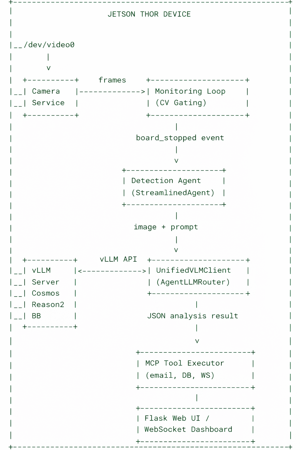
3. System Architecture Overview
The ZEDEDA Camera Monitoring Agent is a multi-layer agentic system. Its key architectural principle is a strict separation between deterministic observation (what is happening in the camera feed) and language-model-directed action (what to do about it).
3.1 The Two-Stage Pipeline Distinction
The system explicitly separates two types of reasoning that are often conflated:
Stage 1: Observation (deterministic, rule-based): Computer vision algorithms compute sensor readings from raw pixels. These are facts, not decisions: “Motion score is 1.2” (below threshold, so board is stationary), “Edge density is 18.3” (board detected in inspection zone), “Board signature is track-7” (this is the same board seen in the prior three frames). No LLM is involved in this stage.
Stage 2: Decision (LLM-directed): Once the deterministic layer confirms that a board is stationary and ready for inspection, the LLM is invoked. The LLM receives the image, the structured prompt, and temporal context. It determines what is wrong with the board, at what confidence level, and what actions to take.
This separation is architecturally important for two reasons:
- Reliability: CV-based gating is fast and deterministic. It filters out the vast majority of frames (empty conveyor, moving boards, blurry images) before they consume VLM inference compute.
- Auditability: Because the LLM makes decisions based on explicit prompt instructions, the reasoning is visible and explainable. The reasoning field in the JSON response is a human-readable account of why the LLM flagged (or cleared) the board.
4. The Monitoring Loop: Deterministic CV Gating
You can view the source code for our ZEDEDA Camera Monitoring Agent on GitHub. In that repo, the MonitoringLoop class (agents/core/monitoring_loop.py) is the sole deterministic component. It runs in a background thread and performs five CV operations on every incoming frame:
4.1 Motion Sensing
Frame-differencing on a downsampled (160×120) grayscale Region of Interest (ROI) computes a motion score as the mean absolute pixel difference between consecutive frames. A configurable threshold (default: 1.8) separates “moving” from “stationary” states. This approach is far cheaper than optical flow and sufficient for the coarse-grained motion discrimination needed here.
4.2 Board Presence Detection
A multi-step segmentation pipeline runs on the ROI:
- Canny edge detection on the blurred ROI.
- Morphological closing and dilation to fill gaps in the PCB outline.
- Contour extraction to find candidate board-shaped objects.
- Scoring each candidate by a weighted combination of area ratio and extent (how rectangular the contour is), filtered by aspect ratio bounds appropriate for PCBs.
The best-scoring candidate is the “board detection.” A hysteresis debouncer (_debounce_presence) requires the board to be detected for N consecutive frames before asserting board_in_zone = True, and absent for M consecutive frames before clearing it. This approach prevents false triggers from partial board entries or momentary occlusions.
4.3 Board Identity Tracking
An IoU-based tracker assigns a persistent track ID to each board as it traverses the inspection zone. When a new board enters (IoU with the previous bbox falls below a threshold while motion is detected), a new track ID is assigned. This track ID is the board’s signature, ensuring that each distinct physical board is inspected at most once, even if it remains stationary for multiple sensing cycles.
If the tracker cannot assign an IoU-based signature (e.g., during startup), a perceptual hash fallback is used: a 32×32 DCT (Discrete Cosine Transform) of the histogram-equalized frame, quantized to bits, and SHA-256 hashed. This hash is stable across minor illumination changes but changes meaningfully when the physical board changes.
4.4 Frame Quality Assessment
The sharpness (Laplacian variance), brightness (mean pixel intensity), and contrast (standard deviation) of the ROI are computed and packed into the Observation object. These quality metrics are forwarded to the LLM as part of the context. The LLM can account for poor frame quality in its confidence estimate; unlike hard quality-gating, this is an advisory signal rather than a filter.
4.5 State Change Detection and the Four-Second Focus Delay
The core loop logic detects a single state transition: the moment when a board’s status changes from “not stopped” to “stopped.” This just_stopped edge trigger fires the LLM inspection. To avoid blurry images caused by camera auto-focus lag (common in consumer USB cameras), the system waits 4 seconds after the board stops before acquiring the inspection frame. This technique is a mechanically-grounded heuristic, not an LLM decision.
Once the settled frame is acquired, _fire_board_ready is called, which invokes the on_board_ready callback registered by the Detection Agent.
5. The VLM Inference Pipeline
5.1 The Unified VLM Client
The UnifiedVLMClient (agents/vlm/client.py) encapsulates all interaction with the VLM inference server. It is responsible for:
- Image encoding: The incoming NumPy frame is resized to a maximum dimension of 1024 pixels (maintaining aspect ratio) before JPEG encoding at 85% quality. Resizing before encoding provides a 40–60% speedup over the encode-then-resize pattern.
- Prompt construction: The prompt is assembled by build_prompt() in agents/vlm/prompts.py. If the user query already embeds a full JSON schema (as indicated by the presence of “detected”: in the text), it is sent verbatim to avoid the “double-schema” confusion that can degrade the reliability of structured output.
- Request routing: All inference requests through the AgentLLMRouter, which provides connection pooling, exponential backoff retries, and global token usage tracking. The router enforces repetition_penalty: 1.15 and frequency_penalty: 0.3 to break degenerate repetition loops in model output. Qwen3-style “thinking mode” is disabled (enable_thinking: False) to ensure the model outputs structured JSON directly.
- Response parsing: A compiled-regex JSON extractor handles common cases: raw JSON, markdown-fenced JSON, and JSON embedded in mixed text. Brace-depth tracking handles nested objects correctly.
- Consistency enforcement: A post-processing step cross-checks the top-level detected boolean against the component-status detail fields. If component fields report “damaged” or “missing” but detected is false, the system overrides to detected = true and logs a warning. This approach corrects a known failure mode in which VLMs correctly fill structured fields but produce an inconsistent top-level flag.
5.2 The PCB Defect Inspection Prompt
The canonical inspection prompt (DEFAULT_MONITORING_DEFECT_PROMPT in agents/vlm/prompts.py) is the single most important artifact in the system. It encodes years of domain knowledge about Arduino Uno R4 Minima inspection in a structured natural-language document:
Component manifest: Lists the expected components (DC barrel-jack, USB-C port, through-hole header pins, QFP microcontroller) with precise physical descriptions (“a chunky, black, cylindrical part that sticks up from the board and NOT flat pads”).
Disambiguation rules: Explicit rules prevent common model confusions. Rule 3 directly addresses a failure mode we observed during development: “Do NOT confuse viewing angle, shadows, or lighting with missing parts.” Rule 4 introduces an “uncertain” category to prevent false positives from occluded areas.
Damage definition: A detailed bulleted list of what “damaged” looks like at the component level: bent metal tabs, tilted housings, cracked plastics, splayed leads. This list is particularly important because the model’s pre-training may have calibrated “damaged” at a coarser granularity than manufacturing acceptance criteria require.
Decision rule: An explicit logical formula maps the per-component status fields to the final detected boolean. This formula separates observation (what you see in each component) from judgment (whether the board passes). The formula can be updated independently of the observation schema.
Output schema: A strict JSON template with typed fields. Requiring a specific output format from the VLM is a form of constrained generation that dramatically improves the reliability of downstream parsing.
5.3 SSIM-Based Frame Deduplication
Between inspections, minor camera jitter or lighting fluctuation may produce nearly identical frames. To avoid redundant VLM calls, the StreamlinedAgent caches the reference frame for each inspection and computes a similarity score against the next frame using structural similarity, SSIM, or, as a faster fallback, normalized template matching. If similarity exceeds 0.95 within a 5-second window, the cached result is reused. The cache is automatically invalidated when the board signature changes, guaranteeing that a new physical board always triggers a fresh inference.
This optimization eliminates a class of redundant inferences that would otherwise inflate latency and token costs without improving defect detection quality.
6. The Proactive Monitoring Loop: A Two-Stage LLM Decision System
For situations requiring adaptive, context-aware monitoring rather than simple trigger-on-stop behavior, the system implements a three-action proactive loop driven by a two-stage LLM pipeline.
6.1 Observation Stage
A dedicated observation prompt (build_proactive_observation_prompt) asks the VLM to act as a perception agent, describing what it sees without making decisions. The output schema captures:
- scene_summary: A natural-language description of the scene.
- target_present / target_state: Whether a PCB is in view and its state (entering, moving, stopped, stable, gone).
- scene_changed: Whether the scene has changed meaningfully since the last observation.
- scene_signature: A consistent identifier for the current board/scene, enabling cross-frame continuity.
- target_ready: Whether the board is in an optimal position for full defect inspection.
The critical design constraint here is stated explicitly in the prompt: “You are observing, NOT deciding. Your observations will inform the decision agent.” This separation prevents the observation stage from second-guessing the decision stage, thereby breaking the principled two-stage architecture.
6.2 Decision Stage
The decision prompt (build_proactive_decision_prompt) presents the observation result, historical context (boards inspected, defects found, time since last action), and the user’s monitoring objective to a separate LLM invocation that selects one of three actions:
| Action | When Used | Resource Cost |
| wait | Scene empty, board moving, or recently inspected | Zero VLM cost |
| quick_check | Confirm board state before committing to full inspection | One fast VLM call |
| full_inspection | Board stable, conditions optimal, defect inspection warranted | Full VLM call + tool execution |
This adaptive action selection is significantly more efficient than a fixed-cadence inspection strategy. On an empty conveyor, the system emits only wait decisions. During a normal production run, most boards receive a quick_check followed by a full_inspection. Only boards with ambiguous states trigger multiple observation-decision cycles.
The decision prompt also includes a scope constraint: if the user instruction is not about monitoring PCB manufacturing defects, the system must refuse, set action=”wait”, and explain the refusal in the reasoning field. This technique is a safety guardrail that prevents the monitoring loop from being repurposed for arbitrary tasks.
6.3 Scope Validation via LLM Classifier
Before the monitoring loop accepts a user instruction, the LLMIntentClassifier (agents/classifiers/llm_classifier.py) is invoked to validate that the instruction falls within the PCB inspection domain. The classifier uses the same vLLM backend as the VLM, but with a text-only prompt that asks it to classify the user’s intent into a domain (pcb or general) and, within the PCB domain, select an appropriate tool from a registry.
The classifier operates with a per-request TTL cache (10 seconds, 128 entries) to avoid redundant LLM calls when the same instruction is validated multiple times within a single request cycle. A lightweight circuit breaker (3 consecutive failures → 30-second backoff) ensures that classifier failures degrade gracefully rather than blocking the monitoring loop.
7. The MCP Tool Execution Layer
The Model Context Protocol (MCP) layer (agents/mcp/) provides a structured interface for the VLM to invoke side-effecting tools after an analysis decision is made. The VLM outputs tool calls as structured JSON in its response text; the executor parses and dispatches them.
7.1 The Agentic Loop
When operating in agentic mode (analyze_agentic in StreamlinedAgent), the VLM analysis and tool dispatch form a multi-round loop (up to 3 rounds by default):
- Round 0: The VLM receives the image and the agentic prompt (which includes available tool schemas). It produces a JSON analysis result and optionally emits tool call blocks in the format tool_call { “tool”: “name”, “arguments”: {…} } .
- Tool execution: The MCP executor dispatches each tool call. Available tools include email notification, event logging to the SQLite database, WebSocket broadcast to the dashboard, and defect recording.
- Continuation: Tool results are concatenated into a continuation prompt. The VLM can inspect the results and decide whether additional tool calls are needed. The loop terminates when no tool calls are emitted or the maximum round count is reached.
This agentic loop means the VLM is not merely a classifier; it is an autonomous actor that can decide to notify engineers, log findings to the database, and broadcast real-time updates to the dashboard, all based on its analysis of the board.
7.2 Agent State Machine
A formal AgentStateMachine (agents/mcp/state_machine.py) governs the agent’s lifecycle with validated transitions:
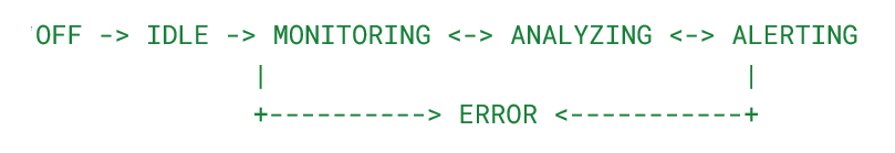
Every state transition is recorded with a timestamp, trigger description, and session ID. This audit trail is exposed via a REST API and can be used for post-incident analysis. Thread safety is enforced via a reentrant lock, ensuring correct behavior when the monitoring loop and web API interact with the state machine concurrently.
8. Infrastructure: vLLM Serving and Kubernetes Deployment
8.1 Why vLLM on Jetson Thor
The NVIDIA Jetson Thor is uniquely positioned for this workload. Its unified memory architecture means the VLM weights and inference buffers reside in a single physical memory pool shared between CPU and GPU, eliminating the PCIe bandwidth bottleneck that limits throughput on discrete-GPU systems. With 32+ GB of unified LPDDR5X memory, the Cosmos Reason 2 8B model fits comfortably alongside the operating system and application stack.
The nvidia/Cosmos-Reason2-8B model is specifically optimized for structured reasoning tasks. It can reliably produce JSON output with nested schemas under constrained-generation prompting, making it well-suited to the structured-output requirements of this inspection pipeline.
vLLM serves the model via the OpenAI-compatible /v1/chat/completions API, enabling the application to swap models transparently. The model_detect.py module queries /v1/models on startup and caches the detected model name, so the application automatically adapts to whatever model the vLLM server is running, with no hardcoded model names in the application code.
8.2 Kubernetes Helm Deployment
The system is packaged as a Helm chart (helm/camera-agent/) that deploys two pods to a K3s cluster:
Camera-agent pod: The Flask application with the proactive monitoring loop. Mounts /dev/video0 via a host device mapping. Exposes a NodePort service on port 30080. Consumes a PVC for persistent data (captured frames, SQLite database, detection images).
vLLM server pod: A NVIDIA Triton Server container with the vLLM Python backend, configured for the Cosmos Reason 2 8B model. Consumes a large PVC (50 Gi) for model weight caching. GPU access is granted via runtimeClassName: nvidia and the NVIDIA device plugin resource request (nvidia.com/gpu: 1).
The two pods communicate via a ClusterIP service (camera-agent-vllm), isolating the inference backend from external network access.
This architecture provides production-grade operational characteristics: rolling updates via helm upgrade, automatic pod restarts on crashes, resource limits and requests, and declarative configuration management.
8.3 The Router Layer
All VLM requests from the application (whether from the detection agent, the proactive loop, or the LLM classifier) pass through a singleton AgentLLMRouter. The router is a thin but important abstraction over the vLLM adapter that provides:
- Connection pooling: Uses a persistent Session to reuse TCP connections.
- Retry with exponential backoff: Transient network errors (common during vLLM model loading) are retried without surfacing errors to the application.
- Concurrency limiting: Prevents request storms from overwhelming the inference server during busy monitoring cycles.
- Token usage tracking: Every request records prompt and completion token counts in a global TokenUsageTracker, exposed via a REST API for cost monitoring.
- Health checking: A check_health() method polls the vLLM server’s /v1/models endpoint, used by the Flask health check route.
9. The Real-Time Dashboard
The Flask application (app/) serves a web-based dashboard over WebSocket and HTTP:
Live camera feed: Frames are streamed to the browser via a WebSocket connection, providing a real-time view of the conveyor. Operators can visually verify that the system is monitoring the correct zone.
Detection log: A scrolling log of recent detection events, each showing the timestamp, detected/cleared status, confidence score, board signature, and the VLM’s reasoning text. This log is the primary interface for operator review.
Proactive monitoring snapshot: A JSON panel showing the current monitoring context: instruction, frames processed, inspections completed, defect count, and the last observation’s sensor readings (motion score, edge density, board-in-zone flag).
Configuration panel: Live configuration updates, such as changing the VLM prompt, adjusting the monitoring instruction, turning email notifications on or off, without restarting the application.
This dashboard is not incidental to the architecture. It is the interface through which operators update the inspection policy (by editing the monitoring instruction) and observe the system’s reasoning (by reading the VLM’s reasoning field). This closing of the human-in-the-loop feedback cycle is what makes prompt-based drift management practical.
10. Comparative Analysis: Prompt Engineering vs. Model Retraining
The following table compares the prompt-engineering approach of this system against conventional model retraining on the dimensions most relevant to industrial deployment:
| Dimension | Model Retraining | Prompt Engineering |
| Adaptation latency | Days to weeks (data collection, annotation, training, validation) | Minutes (edit prompt, apply to running system) |
| Annotation cost | Requires domain-expert annotators for each new class | Domain knowledge expressed directly in natural language by engineers |
| GPU infrastructure required for adaptation | Yes (training cluster) | No (inference server only) |
| Rollback on bad update | Requires reverting model artifacts and redeployment | Edit prompt to prior version; instant effect |
| Audit trail | Model changelog: hard to trace which training images drove a behavior change | Prompt is the policy; every change is diffable text |
| Handling distribution shift | Requires new labeled data from the shifted distribution | Update prompt rules to describe the new visual signatures |
| Handling new board variants | Collect new labeled images; retrain | Update the component manifest in the prompt |
| Handling taxonomy changes | Full relabeling and retraining | Edit the decision rule in the prompt |
| Risk of catastrophic forgetting | High (fine-tuning can degrade prior class performance) | None (base model is frozen) |
| Expertise required | ML engineer + domain expert | Domain expert only |
The trade-off is not cost-free. Prompt engineering has limits:
- Novel visual domains far from pre-training: If the board’s visual appearance is radically different from anything in the VLM’s pre-training distribution, prompting alone cannot compensate.
- Recall vs. precision tuning: Adjusting detection sensitivity (trading precision for recall, or vice versa) can be done via prompt thresholds, but fine-grained calibration may benefit from confidence calibration on a validation set.
- Adversarial failure modes: A VLM may be more susceptible to certain adversarial perturbations than a specialized detector trained on in-distribution data.
For the practical range of drift events encountered in PCB manufacturing, such as board-variant changes, lighting drift, taxonomy updates, and new defect modes, prompt engineering covers the vast majority of cases with dramatically lower operational overhead.
11. Implementation Insights and Engineering Details
11.1 Why Structured JSON Output is Not Trivial
Requiring a VLM to emit valid, schema-conformant JSON is harder than it appears. The model must simultaneously:
- Analyze the image’s visual content.
- Apply the inspection rules from the prompt.
- Fill in all required fields with correctly typed values.
- Produce syntactically valid JSON without markdown artifacts.
Several engineering choices in the system address this:
- Thinking mode disabled: The vLLM request explicitly sets chat_template_kwargs: {“enable_thinking”: False} for models (like Qwen3) that support an extended chain-of-thought reasoning mode. While CoT improves accuracy on complex tasks, it pollutes the output with think tags and reduces the reliability of the JSON output.
- Repetition and frequency penalties: repetition_penalty: 1.15 and frequency_penalty: 0.3 break the degenerate loops where VLMs repeat the same JSON field multiple times.
- Double-schema prevention: The prompt builder checks whether the user query already contains a JSON schema pattern (by searching for “detected”:) before wrapping it in the template. Without this check, the model sees two competing schemas and produces malformed output.
- Consistency enforcement post-processing: Even a well-prompted VLM occasionally produces internally inconsistent output (detailed fields say “damaged,” top-level flag says false). The _enforce_detail_consistency method corrects these cases and logs a warning, making inconsistencies visible without silently discarding valid defect detections.
11.2 Perceptual Hashing for Board Identity
The board signature system solves a subtle but important problem: how do you know whether you are looking at the same board or a different one?
The IoU-based tracker handles the common case (a board enters, stops, and exits while the tracker maintains continuity). The perceptual hash fallback handles edge cases: tracker loss due to occlusion, camera dropout, or system restart.
The hash is computed via:
- Grayscale conversion.
- Histogram equalization (normalization for illumination invariance).
- 32×32 resize.
- 2D DCT.
- Bit quantization of the top-left 8×8 DCT coefficients against their mean.
- SHA-256 of the packed bits, truncated to 24 hex characters.
This algorithm is a classic pHash construction. The histogram equalization step is critical for illumination invariance; without it, a lighting change between two frames of the same board would produce different hashes and trigger redundant inspection.
11.3 Circuit Breaker Pattern for Resilience
Both the VLM client and the LLM classifier implement circuit breaker patterns. When the inference server is unavailable (model loading, transient network failure), the circuit opens after N consecutive failures and returns a graceful fallback response rather than stacking up a queue of failing requests. After a configurable recovery timeout, the circuit half-opens to probe whether the server has recovered.
This pattern is essential for production edge deployment, where the vLLM server may take 10+ minutes to load the model on first boot. The camera agent starts, enters a “wait for inference server” state, and activates automatically once the circuit closes.
12. Deployment Experience on NVIDIA Jetson Thor
12.1 Hardware-Software Co-Design Considerations
The Jetson Thor’s unified memory architecture is well-suited to this workload. The Cosmos Reason 2 8B model requires approximately 16 GB of memory for weights. On a discrete-GPU system, this weight tensor would need to be loaded into GPU VRAM, with activations computed in GPU DRAM and then transferred back to CPU RAM for application processing. On Jetson Thor, the same physical memory is accessible to both CPU and GPU, eliminating this bandwidth bottleneck.
The NVIDIA Container Runtime with JetPack integration ensures that GPU device access is correctly plumbed through Docker containers and K3s pods with no additional configuration. The Helm chart’s runtimeClassName: nvidia annotation is the only Kubernetes-level change needed to enable GPU scheduling.
12.2 Operational Latency Profile
The end-to-end inspection latency (from board-stop event to alert generation) breaks down approximately as follows:
| Stage | Typical Duration | Notes |
| Camera settle delay | 4 seconds | Fixed, allows auto-focus to stabilize |
| Frame acquisition | < 50 ms | USB camera capture |
| SSIM check | < 5 ms | Template matching, skipped if cache miss |
| Image resize + JPEG encode | 20–40 ms | 1024px max dimension, 85% quality |
| vLLM inference (Cosmos Reason 2 8B) | 2–8 seconds | Depends on prompt length, GPU utilization |
| JSON parsing | < 1 ms | Compiled regex, optimized path |
| Tool execution (email + DB) | 100–500 ms | Network-dependent |
| WebSocket broadcast | < 10 ms | Local network |
The dominant latency is the vLLM inference step. For the defect inspection prompt (approximately 700 tokens), Cosmos Reason 2 8B on Jetson Thor typically completes in 2–5 seconds with 0.5 GPU memory utilization. This timeframe is well within the tolerance of most PCB conveyor inspection workflows, where boards dwell in the inspection zone for 5–30 seconds.
12.3 Docker Compose for Development
During development, the system can be run via Docker Compose with the lighter Qwen/Qwen3-VL-4B-Instruct model, which fits in less VRAM and loads faster. The modular prompt architecture means the same inspection prompts work across both models, though Cosmos Reason 2 8B produces more consistent structured JSON output in production.
13. Other Possible Directions
13.1 Retrieval-Augmented Inspection
The current prompt system encodes the component manifest as static text. A natural extension is retrieval-augmented generation (RAG): a database of board variants with component descriptions, defect examples, and historical defect rates. The classifier layer could identify the board variant from the image, retrieve the appropriate component manifest, and dynamically inject it into the inspection prompt. This approach supports arbitrarily large board catalogs without increasing the context window proportionally.
13.2 Feedback-Driven Prompt Refinement
When an operator overrides a VLM decision (clearing a false positive or confirming a missed defect), that feedback can be used to refine the prompt. In the simplest form, a small LLM could analyze the correction and suggest a targeted edit to the inspection rules. Over time, this approach creates a continuous improvement loop where human corrections drive prompt updates, which improve model behavior, which reduces the number of corrections needed.
13.3 Multi-Camera Fusion
The architecture’s camera publisher-subscriber model (services/core/camera.py) supports multiple subscriber IDs per frame source. A natural extension is multi-camera fusion: cameras on multiple sides of the board simultaneously, with the VLM receiving a grid of views and performing holistic defect analysis that accounts for board orientation and component visibility.
13.4 Confidence Calibration and Threshold Learning
The VLM’s confidence scores are outputs of a softmax over logits. They are not guaranteed to be calibrated probabilities. A post-hoc calibration step (Platt scaling or temperature scaling on a small validation set) could convert raw confidence scores into well-calibrated defect probabilities, enabling principled threshold setting with specified false positive rates.
14. Conclusion
The ZEDEDA Camera Monitoring Agent demonstrates that prompt engineering is a viable, production-grade strategy for managing data drift in industrial visual inspection systems. By deploying nvidia/Cosmos-Reason2-8B as a frozen, general-purpose visual reasoner and encoding all domain-specific inspection policy in natural-language prompts, the system achieves:
- Rapid adaptation to new board variants, lighting conditions, and defect taxonomies in minutes rather than weeks.
- No retraining infrastructure required for policy changes; a text editor is sufficient.
- Explainable decisions through the VLM’s natural-language reasoning field.
- Production-grade resilience through circuit breakers, SSIM-based deduplication, and validated state machine transitions.
- Efficient edge deployment on NVIDIA Jetson Thor, exploiting unified memory for cost-effective on-device inference.
The key architectural insight is that VLMs do not lack domain knowledge. Rather, they have absorbed vast amounts of visual and linguistic knowledge during pretraining. What they lack is inspection policy, and that is most naturally expressed and updated in natural language.
In environments where the cost of retraining is measured in engineering weeks, and the pace of change is measured in days, the prompt-first approach is not merely a convenience; it is a competitive advantage.
If you want to build an automated quality inspection agent, whether for electronics or other types of objects, ZEDEDA can help. Our Edge Intelligence Platform combines an AI-driven approach to build and orchestrate edge agents, models, applications, and infrastructure. Our platform lets you build, test, and deploy AI agents and models on any edge hardware, using the same edge orchestration platform trusted by the world’s largest enterprises. Get in touch at https://zededa.com/contact-us/.
References and Technical Specifications
Model: nvidia/Cosmos-Reason2-8B, served via NVIDIA Triton Server with vLLM backend (nvcr.io/nvidia/tritonserver:25.12-vllm-python-py3)
Hardware: NVIDIA Jetson Thor, 32+ GB unified LPDDR5X memory, integrated NVIDIA GPU
Inference framework: vLLM (OpenAI-compatible API, /v1/chat/completions)
Application stack: Python 3.12, Flask, Flask-SocketIO, SQLite, OpenCV, NumPy
Deployment: K3s (lightweight Kubernetes), Helm, NVIDIA Container Runtime, Docker 24.0+
Key algorithmic components: pHash (perceptual hashing for board identity), SSIM / template matching (frame deduplication), Canny + morphological segmentation (board detection), frame-difference motion sensing, IoU tracking, circuit breaker pattern, LLM intent classifier with TTL cache
ZEDEDA Camera Monitoring Agent. AI-Powered PCB Quality Inspection at the Edge. Built for GTC 2025 running on NVIDIA Jetson Thor and Cosmos Reason 2 8B
FAQ
Q: Why use a general-purpose VLM instead of a specialized computer vision model trained specifically for PCB defect detection?
A: A specialized model is more accurate on the distribution it was trained on, but brittle the moment that distribution shifts. A general-purpose VLM like Cosmos-Reason2-8B has already encoded broad visual knowledge about physical objects, materials, and damage patterns during pretraining. The trade-off is that you give up some precision on a fixed task in exchange for dramatically lower adaptation cost when the task changes. For high-mix manufacturing environments where board variants and defect criteria change weekly, that trade-off is almost always worth it.
Q: How does the system handle the case where the VLM’s confidence score is unreliable or poorly calibrated?
A: The current architecture treats confidence scores as advisory signals rather than calibrated probabilities. The decision threshold is configurable without retraining, so operators can tune sensitivity. The post-processing consistency enforcement also catches a known failure mode where the VLM fills component-level detail fields correctly but produces an inconsistent top-level detected flag, overriding it and logging a warning rather than silently dropping the detection.
Q: What prevents the prompt from becoming a maintenance liability as inspection requirements grow more complex?
A: The prompt is structured as a document with distinct sections: component manifest, disambiguation rules, damage definition, decision rule, and output schema. Each of these components has a single, well-defined responsibility. This separation of concerns means that a taxonomy change affects only the decision rule section, and a board variant change affects only the component manifest. The prompt is plain text, so it’s diffable, version-controllable, and reviewable by domain experts without any ML background. That said, prompts can accumulate technical debt like any other artifact, and we suggest feedback-driven prompting,
Q: How does the two-stage observation/decision architecture improve on a single-stage approach?
A: Collapsing observation and decision into one LLM call creates an auditing problem: you can’t tell whether a perception failure caused a wrong decision (the model didn’t see the defect) or a policy failure (the model saw it but applied the wrong acceptance criteria). Separating the stages makes each failure mode independently diagnosable. The observation stage is also cheaper to run, since it can be invoked at a higher frequency on a lighter prompt, while the full inspection prompt is reserved for confirmed ready-state boards. This adaptive action selection (wait / quick_check / full_inspection) is substantially more efficient than fixed-cadence inspection on an active conveyor.
Q: The system uses a 4-second settle delay before capturing the inspection frame. Is there a smarter way to handle camera stabilization?
A: The 4-second delay is a conservative, mechanically-grounded heuristic for USB cameras with slow auto-focus. The more principled approach would be to monitor the sharpness metric (Laplacian variance) computed by the monitoring loop and trigger capture when sharpness stabilizes rather than after a fixed timeout. The current design passes frame-quality metrics (sharpness, brightness, and contrast) to the VLM as advisory context, so the model can account for residual blur in its confidence estimates rather than simply rejecting blurry frames. A smarter settle detection loop is a straightforward extension.
Q: How does the board identity tracking system handle edge cases like occlusion or system restart?
A: The primary tracker uses IoU-based bounding box continuity: when a board’s IoU with the previous detection drops below a threshold. At the same time, motion is detected, a new track ID is assigned. When that fails (occlusion, camera dropout, restart), a perceptual hash fallback kicks in: a histogram-equalized 32×32 DCT of the frame, quantized to bits and SHA-256 hashed. The histogram equalization step is the critical design choice; without it, a lighting change between two frames of the same board would produce different hashes, triggering redundant inspections. The hash is stable across minor variations in illumination but changes meaningfully when the physical board changes.
Q: What are the architectural constraints of running this on Jetson Thor versus a cloud GPU?
A: The key constraint is the memory budget. The Cosmos-Reason2-8B model requires approximately 16 GB for weights, which fits within Jetson Thor’s 128GB unified memory pool, but leaves limited headroom for the OS, application stack, and inference buffers. The unified memory architecture is actually an advantage here: on a discrete-GPU system, you’d pay PCIe bandwidth costs moving activations between CPU and GPU memory. On Jetson, the same physical memory is accessible to both, which improves throughput for memory-bound inference. The operational constraint is cold-start latency, i.e., the vLLM server can take 10+ minutes to load the model on first boot; however, the circuit breaker pattern addresses this constraint by keeping the camera agent in a waiting state rather than failing hard.
Q: How would you extend this architecture to support multiple camera angles or multiple inspection stations?
A: The camera publisher-subscriber model already supports multiple subscriber IDs per frame source, so multi-camera fusion is a natural extension of the existing design rather than a rearchitecture. The VLM would receive a grid of views from multiple angles and perform a holistic analysis, accounting for component visibility and board orientation. For multiple inspection stations, the Kubernetes deployment model scales horizontally, as each station gets its own camera-agent pod, and all stations share the same vLLM server pod via the ClusterIP service, thereby amortizing the model’s cost across stations. The prompt architecture remains the same; only the component manifest and camera configuration differ per station.